Nine circuit topologies, nine flavors of probability art

Every piece in the Quantum Genesis collection starts life as a quantum circuit that runs on a real processor. The chips give us the randomness; the circuit gives us the shape of that randomness. Change how the gates are arranged and you change the probability distribution — which, in a pipeline where the distribution becomes the seed, changes the art.

I went through nine basic topologies before one stuck. Some were dead ends, some were fascinating in ways I didn't want in a collection, and one became the exact circuit behind all 100 pieces. Here's what each one does to the maths, and what that does to the visuals.

Spoiler for the ending: the topology that won is not the one I expected when I started.

What a topology actually controls

A quantum circuit topology is just the specific arrangement of gates over the qubits: which gates, where, in what order, and how qubits connect to one another through entanglement.

Two circuits with the same qubit count but different gate arrangements produce completely different measurement distributions. In generative art terms, that means different color palettes, different structural patterns, different textures. The topology is the composer; the hardware is the instrument.

For the collection, we ran 100 circuits on real hardware — Origin Quantum's WK_C180 (180 qubits) and IBM Quantum's ibm_fez (156 qubits). The measurement outcomes became SHA-256 seeds that drove every visual parameter of each NFT.

The circuit everything starts from

The foundation is deliberately simple. Apply a Hadamard gate (H) to every qubit, putting each into an equal superposition of |0⟩ and |1⟩. Chain CNOT gates between qubits to entangle them. Measure everything.

The Hadamard layer creates maximum uncertainty. The CNOT layer introduces correlations. The specific CNOT pattern — the topology — decides what kind of correlations show up in the measurement data. That's the whole lever.

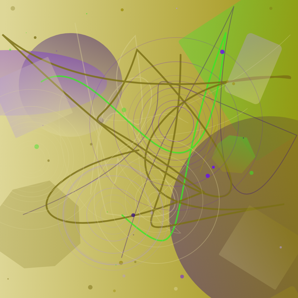
The nine topologies, from noise to structure

1. All-Hadamard (uniform superposition)

H on every qubit, then measure. No entanglement at all. Each qubit is independently 50/50, so you get a uniform distribution over all 2^n bitstrings.

Visual effect: maximum randomness. The art trends toward pure noise — no structure, no patterns. Useful as a baseline and, on its own, genuinely boring.

2. GHZ state (maximally entangled)

H on qubit 0, then CNOT from qubit 0 to every other qubit. That builds the Greenberger-Horne-Zeilinger state — a superposition of all-zeros and all-ones. Measurement collapses to 000...0 or 111...1 with equal probability.

Visual effect: extremely binary. Stark contrast between two dominant modes, very little middle ground. Bold, but there are only two notes in the song.

3. Linear CNOT chain (nearest-neighbor)

CNOT from qubit 0→1, then 1→2, then 2→3, onward. Each qubit entangles only with its immediate neighbor, and correlations decay with distance.

Visual effect: gradient-like. Adjacent regions of the art correlate; distant regions diverge. Smooth transitions and organic-feeling patterns.

4. Steane-7 code topology (error-correction inspired)

Based on the [[7,1,3]] quantum error-correcting code. Specific CNOT patterns link 7 qubits in a redundancy-oriented structure, then repeat to 12 qubits.

Visual effect: highly structured with repeating motifs. The redundancy baked into error-correcting codes creates self-similar patterns in the distribution — fractal-like repetition.

5. Alternating CNOT (even-odd pattern)

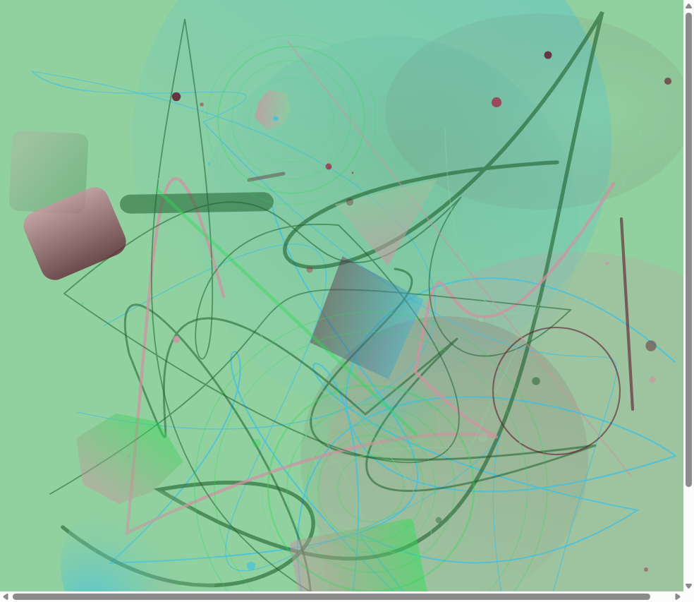
First layer: CNOT on (0,1), (2,3), (4,5), etc. Second layer: CNOT on (1,2), (3,4), (5,6), etc. This is the topology the collection actually uses.

Visual effect: balanced entanglement without GHZ's extremes or a linear chain's locality. Rich distributions with both local correlations and longer-range structure. The sweet spot for generative art.

6. Random rotation angles (parameterized Ry gates)

Instead of uniform Hadamards, apply Ry(θ) with different angles per qubit before the CNOT layer. Every qubit starts in a different superposition bias.

Visual effect: asymmetric distributions. Some outcomes become much more likely than others, producing dominant colors or structural biases. Parametrically unique on every run.

7. Grover-inspired amplitude amplification

The Grover diffusion structure: H layer, conditional phase flip, H layer again. Not a full search, but the amplitude amplification concentrates probability on specific bitstrings.

Visual effect: peaked distributions with one or a few outcomes dominating. Strong focal points surrounded by subtle variation. Dramatic, high-contrast.

8. W-state preparation

The W state: an equal superposition of all single-excitation states (100...0 + 010...0 + 001...0 + ...). Exactly one qubit is |1⟩ in each term. It needs a specific sequence of controlled rotations and CNOTs.

Visual effect: sparse distributions. Most bitstrings have zero probability. W-state art is minimalist — a few dominant elements on a clean background. Elegant and restrained, but not what you want across 100 pieces.

9. Bell pair cascade

Independent Bell pairs: (0,1), (2,3), (4,5), etc. Each pair is maximally entangled internally but independent of the others. A modular approach to entanglement.

Visual effect: blocky and segmented. Each Bell pair contributes one correlated bit pair, so the art tiles into distinct regions with internal coherence and no global pattern.

Where the interesting middle lives

The connection between topology and visuals isn't metaphorical; it's mathematical. Each topology produces a specific probability distribution over 2^12 = 4,096 outcomes for a 12-qubit circuit.

Run thousands of shots (8,000 on Origin Quantum, 4,096 on IBM Quantum) and you get a histogram of measurement frequencies. That histogram becomes the seed data. High-frequency outcomes drive the art's structure; rare outcomes add texture and detail.

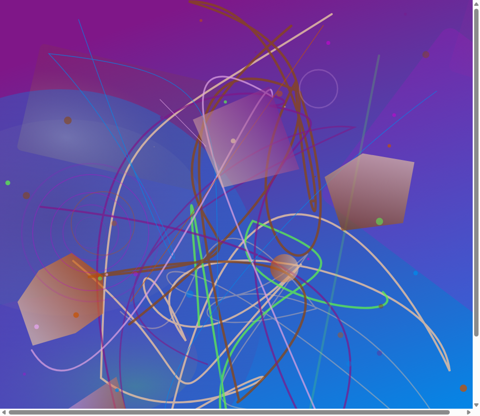
> The variable that matters most is entanglement. No entanglement produces noise. Maximum entanglement (GHZ) produces binary extremes. The interesting art lives in the middle — partial entanglement with complex correlation structures.

The alternating CNOT topology hits exactly that middle. Enough entanglement for structure, enough independence for variety, enough complexity for visual richness. That's why all 100 Quantum Genesis pieces use it.

The exact circuit behind the collection

Every NFT ran this 12-qubit circuit:

1. Hadamard layer: H gate on all 12 qubits (q0 through q11)
2. Even CNOT layer: CNOT(q0,q1), CNOT(q2,q3), CNOT(q4,q5), CNOT(q6,q7), CNOT(q8,q9), CNOT(q10,q11)
3. Odd CNOT layer: CNOT(q1,q2), CNOT(q3,q4), CNOT(q5,q6), CNOT(q7,q8), CNOT(q9,q10)
4. Measurement: all 12 qubits into classical bits

NFTs #1–18 ran on Origin Quantum's WK_C180 (180 qubits) with 8,000 shots via pyqpanda3. NFTs #19–100 ran on IBM Quantum's ibm_fez and ibm_torino (156q/133q) with 4,096 shots via Qiskit Runtime's SamplerV2.

The code, which is short on purpose

from qiskit import QuantumCircuit
import hashlib

def build_nft_seed_circuit(n_qubits=12):
    """Build a max-entropy seed-generation circuit.
    H on all qubits + alternating CNOT chains + measure all."""
    qc = QuantumCircuit(n_qubits, n_qubits)

    # Hadamard layer — uniform superposition
    for i in range(n_qubits):
        qc.h(i)

    # Even CNOT layer
    for i in range(0, n_qubits - 1, 2):
        qc.cx(i, i + 1)

    # Odd CNOT layer
    for i in range(1, n_qubits - 1, 2):
        qc.cx(i, i + 1)

    # Measure all qubits
    qc.measure(range(n_qubits), range(n_qubits))
    return qc

def counts_to_seed(counts):
    """Convert measurement counts to a deterministic hex seed via SHA-256."""
    sorted_counts = sorted(counts.items())
    raw = "|".join(f"{k}:{v}" for k, v in sorted_counts)
    return hashlib.sha256(raw.encode()).hexdigest()

The circuit is deliberately simple. The complexity isn't designed into the gates; it comes out of the hardware — gate errors, decoherence, crosstalk, and the genuine randomness of quantum measurement.

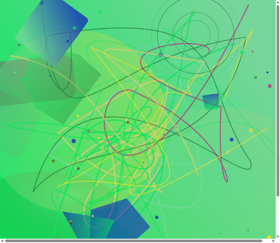
Every piece in the collection is a frozen quantum measurement. The topology shaped the probability space; the hardware collapsed it; the art is what came out. If you've played with different gate arrangements in Qiskit, tell me which one surprised you — because the GHZ one certainly surprised me, and not in a good way.