Building the Quantum Genesis art generator: from measurement seed to SVG
Quantum Genesis is 100 pieces of abstract art, and no human picked a single color or arranged a single shape. Every attribute was determined by a Python script fed with random data from real quantum measurements on IBM's ibm_fez and Origin Quantum's WK_C180. The machine hands back a probability distribution; the script turns that into a layered SVG composition.
This post is the complete walkthrough of how that generator works — every layer of the composition, and enough code to build your own. If you're not interested in quantum hardware, the generator itself is fully portable to any random source; everything down to random.seed(42) behaves the same.
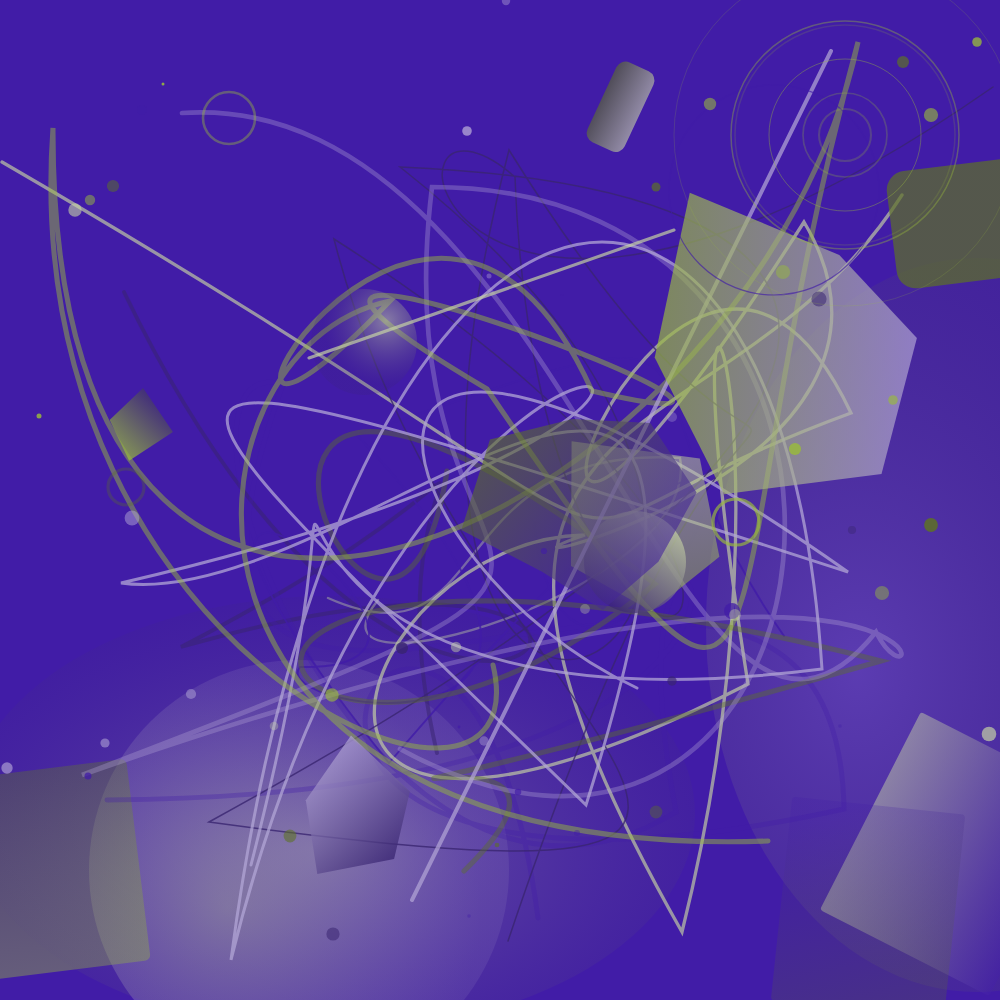
The pipeline: seeds to SVG
Four stages:
Quantum Computer → Raw Measurements (4096 shots)
    → SHA-256 Hash (256-bit seed)
        → Python QuantumRNG (deterministic from seed)
            → SVG Artwork (layered composition)
The quantum computer produces a probability distribution from 4096 measurement shots. We hash that distribution into a 256-bit seed. From the seed, a deterministic PRNG produces every random value the artwork needs. So the art is reproducible from the seed — but the seed itself is unreproducible, because it came from a real quantum measurement.
Color theory: HSL and harmony types
Random RGB values produce muddy, clashing palettes. We work in HSL (Hue, Saturation, Lightness) and use established color harmony rules so the palettes land somewhere pleasant:
class ColorHarmony:
    """Generate harmonious color palettes from a base hue."""

    @staticmethod
    def complementary(base_hue: float) -> list[float]:
        """Two colors opposite on the wheel (180° apart)."""
        return [base_hue, (base_hue + 180) % 360]

    @staticmethod
    def analogous(base_hue: float) -> list[float]:
        """Three colors adjacent on the wheel (±30°)."""
        return [
            (base_hue - 30) % 360,
            base_hue,
            (base_hue + 30) % 360
        ]

    @staticmethod
    def triadic(base_hue: float) -> list[float]:
        """Three colors equally spaced (120° apart)."""
        return [
            base_hue,
            (base_hue + 120) % 360,
            (base_hue + 240) % 360
        ]

    @staticmethod
    def split_complementary(base_hue: float) -> list[float]:
        """Base + two colors adjacent to its complement."""
        return [
            base_hue,
            (base_hue + 150) % 360,
            (base_hue + 210) % 360
        ]

    @staticmethod
    def tetradic(base_hue: float) -> list[float]:
        """Four colors forming a rectangle on the wheel."""
        return [
            base_hue,
            (base_hue + 90) % 360,
            (base_hue + 180) % 360,
            (base_hue + 270) % 360
        ]
The quantum seed decides which harmony type to use and what the base hue is. Saturation and lightness vary per element but stay inside ranges that avoid washed-out or murky output:
# Saturation: 50-90% (vibrant but not neon)
# Lightness: 35-75% (visible against both light and dark backgrounds)
saturation = 50 + rng.random() * 40
lightness = 35 + rng.random() * 40
The QuantumRNG bridge
This is the deterministic PRNG seeded by the quantum measurement hash — the thing that makes each piece reproducible:
import hashlib
import struct

class QuantumRNG:
    """Deterministic RNG seeded by quantum measurement data."""

    def __init__(self, seed_hex: str):
        """
        Args:
            seed_hex: 64-char hex string (SHA-256 of quantum measurements)
        """
        self.seed = int(seed_hex, 16)
        self.state = self.seed
        self.calls = 0

    def random(self) -> float:
        """Return a float in [0, 1)."""
        # xorshift128+ algorithm
        self.state ^= (self.state << 13) & ((1 << 256) - 1)
        self.state ^= (self.state >> 17)
        self.state ^= (self.state << 5) & ((1 << 256) - 1)
        self.calls += 1
        # Take lower 53 bits for double precision
        return (self.state & ((1 << 53) - 1)) / (1 << 53)

    def randint(self, a: int, b: int) -> int:
        """Return integer in [a, b] inclusive."""
        return a + int(self.random() * (b - a + 1))

    def choice(self, items: list):
        """Pick a random element from a list."""
        return items[self.randint(0, len(items) - 1)]

    def gauss(self, mu: float, sigma: float) -> float:
        """Approximate Gaussian using Box-Muller transform."""
        import math
        u1 = max(self.random(), 1e-10)
        u2 = self.random()
        return mu + sigma * math.sqrt(-2 * math.log(u1)) * math.cos(2 * math.pi * u2)
The key property: it's deterministic. The same seed produces the same number sequence, and thus the same artwork. But the seed came off a quantum computer, so it's genuinely random and unreproducible on its own.
The SVG canvas
We generate SVG rather than rasters — it's resolution-independent, compresses well, and is trivial to produce programmatically:
def create_svg(width: int = 1000, height: int = 1000) -> str:
    """Create the SVG document wrapper."""
    return f'''<svg xmlns="http://www.w3.org/2000/svg"
     viewBox="0 0 {width} {height}"
     width="{width}" height="{height}">
  <defs>
    <!-- Gradients and filters defined here -->
  </defs>
  <!-- Layers inserted here -->
</svg>'''
The canvas is 1000x1000, and the composition builds back to front:
- Background gradient
- Large geometric shapes (circles, rectangles, polygons)
- Bezier curves (flowing organic lines)
- Mid-ground elements (smaller shapes, rings)
- Particles (tiny dots and marks)
- Noise texture overlay
Layer 1: background and gradients
The background sets the mood. We use radial and linear gradients from the harmony palette:
def generate_background(rng: QuantumRNG, palette: list) -> str:
    """Generate background with gradient."""
    bg_type = rng.choice(["radial", "linear", "dual"])
    c1 = palette[0]
    c2 = palette[1 % len(palette)]

    if bg_type == "radial":
        cx = 30 + rng.random() * 40  # Center 30-70%
        cy = 30 + rng.random() * 40
        return f'''
        <defs>
          <radialGradient id="bg" cx="{cx}%" cy="{cy}%"
                          r="70%" fx="{cx}%" fy="{cy}%">
            <stop offset="0%" stop-color="hsl({c1},70%,15%)" />
            <stop offset="100%" stop-color="hsl({c2},60%,8%)" />
          </radialGradient>
        </defs>
        <rect width="1000" height="1000" fill="url(#bg)" />'''

    elif bg_type == "linear":
        angle = rng.randint(0, 360)
        return f'''
        <defs>
          <linearGradient id="bg" gradientTransform="rotate({angle})">
            <stop offset="0%" stop-color="hsl({c1},65%,12%)" />
            <stop offset="100%" stop-color="hsl({c2},55%,6%)" />
          </linearGradient>
        </defs>
        <rect width="1000" height="1000" fill="url(#bg)" />'''

    else:  # dual gradient
        return f'''
        <rect width="1000" height="1000" fill="hsl({c1},50%,10%)" />
        <rect width="1000" height="1000"
              fill="hsl({c2},40%,20%)" opacity="0.3"
              rx="200" ry="200" />'''
Backgrounds stay dark (lightness 6-15%) so the vibrant elements on top pop. Dark grounds add drama and make colors feel more intense.
Layer 2: geometric shapes
This layer drops 5-15 large shapes, each with randomized position, size, color, rotation, and opacity:
def generate_shapes(rng: QuantumRNG, palette: list, count: int) -> str:
    """Generate geometric shapes layer."""
    shapes = []
    for _ in range(count):
        shape_type = rng.choice(["circle", "rect", "polygon", "ring"])
        x = rng.random() * 1000
        y = rng.random() * 1000
        hue = rng.choice(palette)
        sat = 50 + rng.random() * 40
        lit = 40 + rng.random() * 30
        opacity = 0.1 + rng.random() * 0.5
        color = f"hsl({hue},{sat}%,{lit}%)"

        if shape_type == "circle":
            r = 30 + rng.random() * 150
            shapes.append(
                f'<circle cx="{x}" cy="{y}" r="{r}" '
                f'fill="{color}" opacity="{opacity:.2f}" />'
            )
        elif shape_type == "rect":
            w = 40 + rng.random() * 200
            h = 40 + rng.random() * 200
            angle = rng.random() * 360
            shapes.append(
                f'<rect x="{x}" y="{y}" width="{w}" height="{h}" '
                f'fill="{color}" opacity="{opacity:.2f}" '
                f'transform="rotate({angle:.1f},{x},{y})" rx="5" />'
            )
        elif shape_type == "polygon":
            sides = rng.randint(3, 8)
            radius = 40 + rng.random() * 120
            points = []
            for i in range(sides):
                angle = (360 / sides) * i + rng.random() * 20
                px = x + radius * math.cos(math.radians(angle))
                py = y + radius * math.sin(math.radians(angle))
                points.append(f"{px:.1f},{py:.1f}")
            shapes.append(
                f'<polygon points="{" ".join(points)}" '
                f'fill="{color}" opacity="{opacity:.2f}" />'
            )
        else:  # ring
            r = 40 + rng.random() * 100
            sw = 2 + rng.random() * 8
            shapes.append(
                f'<circle cx="{x}" cy="{y}" r="{r}" '
                f'fill="none" stroke="{color}" '
                f'stroke-width="{sw:.1f}" opacity="{opacity:.2f}" />'
            )

    return "\n".join(shapes)
The low opacities (0.1-0.6) are the point. When semi-transparent shapes overlap they produce emergent colors and depth that neither shape has alone — the layering is what gives generative art its characteristic richness.
Layer 3: bezier curves and flow fields
Bezier curves add the organic, flowing quality that keeps computer-generated art from feeling rigid:
def generate_bezier_curves(rng: QuantumRNG, palette: list, count: int) -> str:
    """Generate flowing bezier curves."""
    curves = []
    for _ in range(count):
        hue = rng.choice(palette)
        sat = 60 + rng.random() * 30
        lit = 50 + rng.random() * 25
        color = f"hsl({hue},{sat}%,{lit}%)"
        sw = 1 + rng.random() * 4
        opacity = 0.2 + rng.random() * 0.6

        # Start point
        sx, sy = rng.random() * 1000, rng.random() * 1000

        # Build a path with multiple cubic bezier segments
        segments = rng.randint(2, 5)
        path = f"M {sx:.1f} {sy:.1f}"

        cx, cy = sx, sy
        for _ in range(segments):
            # Control point 1: offset from current position
            cp1x = cx + rng.gauss(0, 150)
            cp1y = cy + rng.gauss(0, 150)
            # Control point 2: offset from endpoint
            ex = cx + rng.gauss(0, 200)
            ey = cy + rng.gauss(0, 200)
            cp2x = ex + rng.gauss(0, 100)
            cp2y = ey + rng.gauss(0, 100)

            path += f" C {cp1x:.1f} {cp1y:.1f}, {cp2x:.1f} {cp2y:.1f}, {ex:.1f} {ey:.1f}"
            cx, cy = ex, ey

        curves.append(
            f'<path d="{path}" fill="none" stroke="{color}" '
            f'stroke-width="{sw:.1f}" opacity="{opacity:.2f}" '
            f'stroke-linecap="round" />'
        )

    return "\n".join(curves)
We use Gaussian-distributed offsets (rng.gauss) for the control points, not uniform random. Gaussian gives gentle, natural flow with the occasional dramatic sweep; uniform random produces jumpy zigzags.
Some pieces instead use a flow field, where curves follow a noise gradient and form coherent patterns like wind or water:
def noise_2d(x: float, y: float, seed: int) -> float:
    """Simple value noise for flow fields."""
    # Hash-based noise (not true Perlin, but fast and good enough)
    n = int(x * 7 + y * 13 + seed * 31) & 0xFFFF
    n = (n * 15731 + 789221) & 0x7FFFFFFF
    return (n / 0x7FFFFFFF) * 2 - 1

def generate_flow_field(rng: QuantumRNG, palette: list) -> str:
    """Generate curves that follow a noise field."""
    lines = []
    num_lines = rng.randint(20, 50)
    noise_seed = rng.randint(0, 10000)

    for _ in range(num_lines):
        x = rng.random() * 1000
        y = rng.random() * 1000
        hue = rng.choice(palette)
        color = f"hsl({hue},{60 + rng.random()*30}%,{50 + rng.random()*20}%)"

        points = [f"M {x:.1f} {y:.1f}"]
        for step in range(30):
            angle = noise_2d(x / 200, y / 200, noise_seed) * math.pi * 2
            x += math.cos(angle) * 8
            y += math.sin(angle) * 8
            points.append(f"L {x:.1f} {y:.1f}")

        path = " ".join(points)
        lines.append(
            f'<path d="{path}" fill="none" stroke="{color}" '
            f'stroke-width="1.5" opacity="0.4" stroke-linecap="round" />'
        )

    return "\n".join(lines)
Layer 4: particles and noise texture
The particle layer adds texture and depth — hundreds of tiny dots scattered like stars or dust:
def generate_particles(rng: QuantumRNG, palette: list, count: int) -> str:
    """Generate particle scatter."""
    particles = []
    for _ in range(count):
        x = rng.random() * 1000
        y = rng.random() * 1000
        r = 0.5 + rng.random() * 3
        hue = rng.choice(palette)
        lit = 60 + rng.random() * 30
        opacity = 0.2 + rng.random() * 0.6

        particles.append(
            f'<circle cx="{x:.1f}" cy="{y:.1f}" r="{r:.1f}" '
            f'fill="hsl({hue},70%,{lit}%)" opacity="{opacity:.2f}" />'
        )

    return "\n".join(particles)
For the noise texture we use an SVG filter that lays down subtle grain:
def generate_noise_filter() -> str:
    """SVG filter for subtle noise texture."""
    return '''
    <filter id="noise">
      <feTurbulence type="fractalNoise" baseFrequency="0.65"
                     numOctaves="3" stitchTiles="stitch" />
      <feColorMatrix type="saturate" values="0" />
    </filter>
    <rect width="1000" height="1000" filter="url(#noise)"
          opacity="0.05" />'''
At 5% opacity the noise overlay adds analog film-like grain that softens the digital precision of the vector shapes.
Putting it together
The main generator orchestrates all the layers:
import math

def generate_artwork(seed_hex: str, token_id: int) -> str:
    """Generate complete SVG artwork from quantum seed."""
    rng = QuantumRNG(seed_hex)

    # Choose color harmony
    base_hue = rng.random() * 360
    harmony_type = rng.choice([
        "complementary", "analogous", "triadic",
        "split_complementary", "tetradic"
    ])
    harmony_fn = getattr(ColorHarmony, harmony_type)
    palette = harmony_fn(base_hue)

    # Determine complexity (driven by quantum entropy)
    num_shapes = rng.randint(5, 15)
    num_curves = rng.randint(3, 10)
    num_particles = rng.randint(50, 300)
    use_flow_field = rng.random() > 0.6

    # Build SVG layers
    bg = generate_background(rng, palette)
    shapes = generate_shapes(rng, palette, num_shapes)
    if use_flow_field:
        curves = generate_flow_field(rng, palette)
    else:
        curves = generate_bezier_curves(rng, palette, num_curves)
    particles = generate_particles(rng, palette, num_particles)
    noise = generate_noise_filter()

    # Compose final SVG
    svg = f'''<svg xmlns="http://www.w3.org/2000/svg"
     viewBox="0 0 1000 1000" width="1000" height="1000">
  <!-- Quantum Genesis #{token_id} -->
  <!-- Seed: {seed_hex[:16]}... -->
  <!-- Harmony: {harmony_type} | Base hue: {base_hue:.0f}° -->
  {bg}
  <g id="shapes">{shapes}</g>
  <g id="curves">{curves}</g>
  <g id="particles">{particles}</g>
  {noise}
</svg>'''

    return svg
Each artwork takes about 50ms to generate. The quantum measurement that feeds it took ~19 seconds per NFT on IBM's ibm_fez. Generating the art is the fast part — nearly all the time goes into securing the seed.
What the full run produced
Each piece is unique not just in the "different random seed" sense but structurally. The measurements determine the color harmony type (5 possibilities), base hue (360 degrees), shape count (5-15), shape types, curve style (bezier or flow field), particle density (50-300), and every position, size, rotation, and opacity. Two seeds differing by a single bit produce completely different artworks.
That raises the natural question: what makes the quantum source special when you could seed this with math.random() and get something that looks similar?
- Provenance. Each seed is cryptographically linked (via SHA-256) to a specific circuit run on a specific processor at a specific time. That's verifiable on-chain.
- True randomness. Classical PRNGs are deterministic — know the state and you can predict everything after. Quantum measurements are fundamentally random by the laws of physics.
- Unreproducibility. You cannot re-run the same circuit on the same processor and recover the same measurements. Calibration drift, thermal noise, and quantum indeterminacy guarantee it.
The generator is identical for all 100 pieces. What makes each one distinct is the seed — and that seed comes from the universe itself. I went deeper on why that randomness behaves so differently from PRNG output in the quantum-randomness post, and the pipeline that rasterizes these SVGs to PNG is covered in the headless-Chrome conversion post.
Build your own
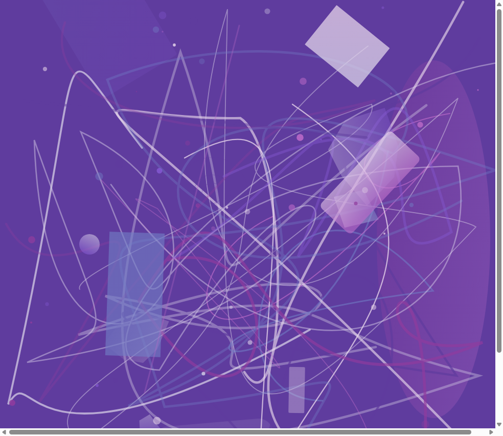
You don't need a quantum computer to experiment with generative art. Start with random.seed(42) and swap in a quantum source later — the techniques above work with any random source. The full Qiskit circuits that produced our seeds are covered in the quantum RNG writeup, and I published a condensed narrative on Dev.to. If you build your own and discover a harmony or layer trick I missed, I'd love to see it.


Comments
Post a Comment